Four Ingredients for Successful Language Model Retrofitting
Retrofitting enables GPU-poor people (like most of us) to do language model architecture research without falling very far off the frontier of the best open models since the cost of retrofitting an existing model is a small fraction of the cost of training a new model from scratch. Even if you do have the budget to train from scratch, retrofitting could give you a substantially faster pace of new insights.
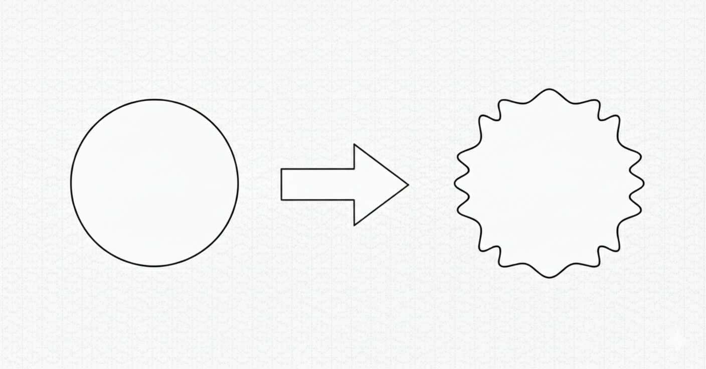
While language model fine-tuning is super common nowadays and there is plenty of wisdom on how to fine-tune well (such as using parameter-efficient methods), retrofitting receives a lot less attention. When we fine-tune a model, we change the values of some of the model parameters. When retrofitting, we change the values of the parameters and the model architecture, in other words which parameters there are.
Retrofitting is very cool, and more people should use it to do research. It is also very broadly useful across different areas. For example, we can retrofit language models to lower-precision parameters via Quantization-Aware Training (QAT), to use a more lightweight KV cache via KV cache sparsification, or to predict multiple future tokens concurrently via Multi-Token Prediction.
My own research usually involved retrofitting to change the tokenizer, for example to an arbitrary unseen tokenizer or recently to byte-level tokenization.
Over time, I’ve noticed a couple of common ingredients across successful retrofitting projects, which I wanted to share here. Use the original version of the model as a teacher (self-distillation). Gradually move from the original architecture to the target architecture (architecture-space graduality). Match the expressivity of the original architecture and the new architecture and be careful about the data coverage of the retrofitting procedure.
Self-Distillation
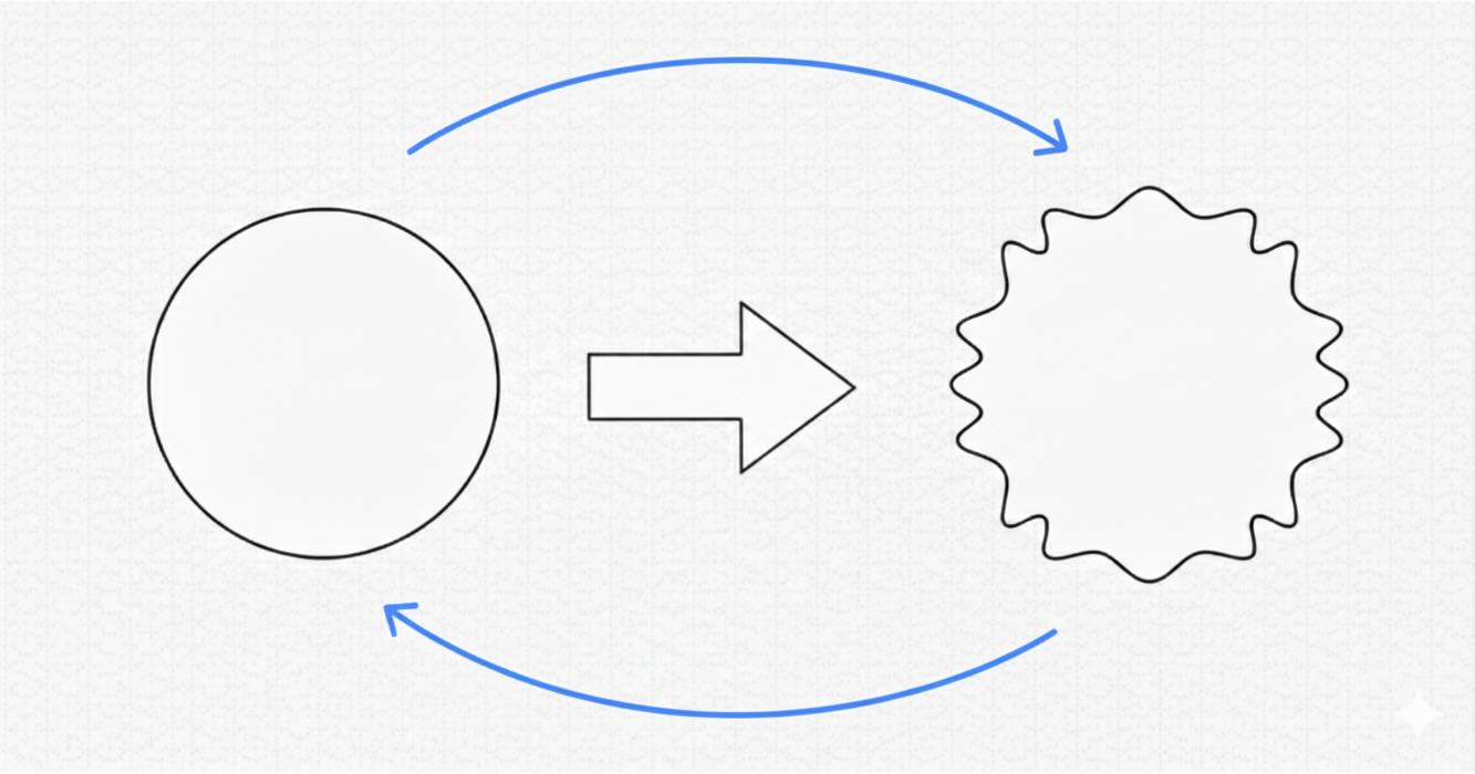
Distillation transfers knowledge from a teacher model to a student model. In the LLM case, this is often done by minimizing the KL divergence between their token predictions. Self-distillation is distillation where the teacher and the student have originally been the same model, but the student has undergone some change. You’re most likely to encounter self-distillation in RL post-training these days, where the objective can often look something like this:
\[\begin{equation*} \max_{\pi_\theta} \mathbb{E}_{x \sim \mathcal{D},\, y \sim \pi_\theta(y \mid x)} \left( r_\phi(x, y) - \textcolor{green}{\beta \, \mathrm{KL}\!\left( \pi_\theta(y \mid x)\,\|\,\pi_{\mathrm{ref}}(y \mid x) \right)} \right) \end{equation*}\]Here, \(r_\phi(x, y)\) is some task reward and \(\textcolor{green}{\beta \, \mathrm{KL}\!\left(\pi_\theta(y \mid x)\,\|\,\pi_{\mathrm{ref}}(y \mid x)\right)}\) is a KL divergence term penalising drift of the model being post-trained (the student) from the model before this post-training step (the teacher). This is self-distillation. In the case of retrofitting, we often do not even have a term like \(r_\phi(x, y)\). Our goal is purely for our model after the architecture change to perform as well as the model before the architecture change. Self-distillation is a really natural fit here.
If you just remember one thing from this blog post, it should be to use self-distillation. This has the single biggest impact on retrofitting success in my experience, and it’s usually pretty easy to implement. However, there are some details to be aware of.
On-Policy vs. Off-Policy
The above example from RL fine-tuning is on-policy self-distillation. On-policy means that the data we compute the KL on is generated by the current version of the student at every training step. Unfortunately, using on-policy data is often tricky since it requires a fast way to sample from the student in the training loop. However, in my experience, using a different source of data instead of data generated by the current student (being off-policy) already provides huge benefits over retaining the model’s pretraining objective.
\[\text{on-policy self-distillation} > \text{off-policy self-distillation} \gg \text{no self-distillation}\]As an example, let’s say we want to make our model faster by quantizing it. The model should retain its original behaviour to the extent possible. We can very easily do off-policy self-distillation by choosing some dataset (for example, web-style pretraining data) and for every batch, first computing the logits of the original unquantized model (the teacher) and the quantized model (the student), then updating our quantized model via the KL divergence gradients of the student logits to the teacher logits.
Exactness
An important property of a self-distillation objective is exactness: the objective should be minimal if and only if the retrofitted model behaves exactly like the original model. Otherwise the optimisation process can converge to solutions that aren’t what we want. This is often trivial. For example, KL divergence is exact in this sense, irrespective of whether we are on- or off-policy. However, exactness is not always trivial: if we change the tokenizer (i.e., the student and the teacher end up using different tokenizers), we can not use standard KL. In this case, exactness of the objective is not so easy to achieve, but luckily we wrote a paper doing so. Exactness also becomes more important to consider when we supplement our main objective such as KL with auxiliary losses which may improve performance on some task but remove exactness (which is not to say that this is necessarily bad, but it’s an important tradeoff!).
Why self-distillation? Shouldn’t the teacher be larger than the student?
Let’s say a larger model from the same family is available. Shouldn’t we use this model as a teacher? Potentially yes, but there is some evidence that larger models do not always make better teachers, and a teacher which is too large can actually lead to worse performance of a student trained on it. Additionally, larger teachers require more compute. In my experience, using the model itself as the teacher via self-distillation usually provides the best tradeoff, but this may not always be the case.
Architecture-Space Graduality
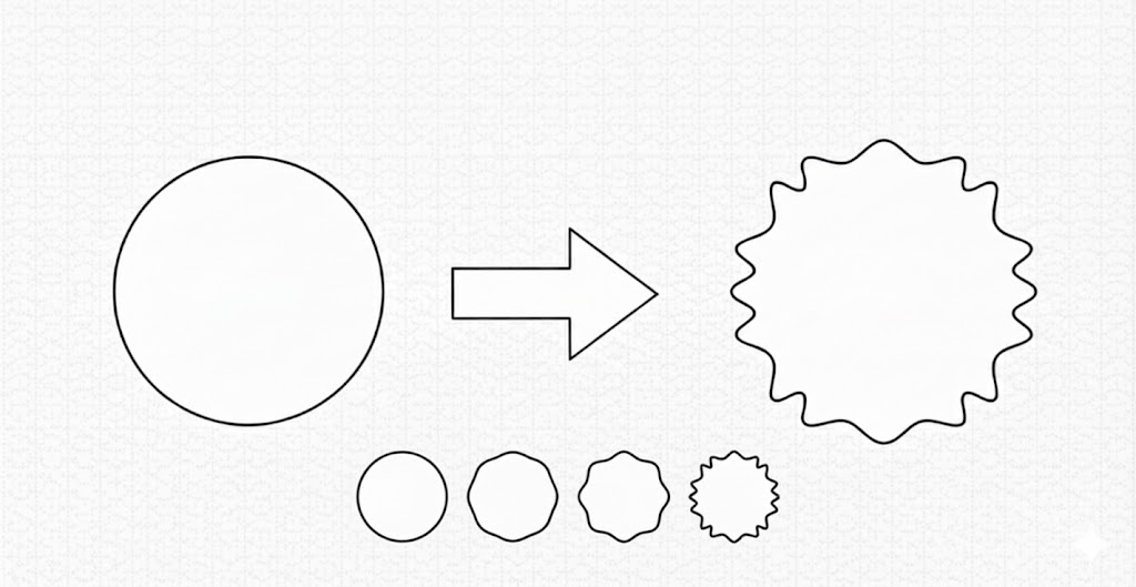
If our change to the model architecture is too large, doing it all at once can catastrophically break the model. We can instead gradually move from the original model’s architecture to the target architecture. Graduality is less well-established than self-distillation, but there is growing evidence that it can be useful. For example, gradually removing LayerNorms can create a LayerNorm-Free model, gradually increasing KV cache sparsity can create faster models and byte-level models can gradually learn to compress their inputs more strongly. Graduality is very interesting for a couple of reasons.
First, the architecture space is typically discrete. It’s not really intuitive to think of ‘2/3rds of a layer’ or ‘half a LayerNorm’, so interpolation between architectures is tricky. The effectiveness of graduality depends to a large extent on how well we can define a gradual process over the discrete architecture space. To make this clearer, let’s think of an example of the ‘wrong kind’ of graduality. We have a version of the model which has undergone some architecture change (for example, quantization). To gradually move our architecture toward this model, we can consider our student to be an ensemble of this model and the original model, with the logits at the start of training being given purely by the original model, and then throughout training gradually moving toward the logits of the quantized model. This fulfils our goal of conducting a gradual change, and the model at the final training step being equivalent to our target model. However, I would not expect this type of graduality to help us; the success of graduality seems in some way contingent on the ‘fine-grainedness’ with which we can interpolate between the two architectures.
Second, there is no free lunch through graduality. Every training step we spend on an architecture which is in-between our original architecture and the final architecture is one training step we do not spend on the final architecture. In other words, moving gradually makes our final goal less in-distribution.
There is an interesting connection between architecture-space graduality and curriculum learning, where a model is trained on easier data first and training gradually moves toward harder examples. I am not aware of successful applications of curriculum learning in modern LLMs.
Expressivity
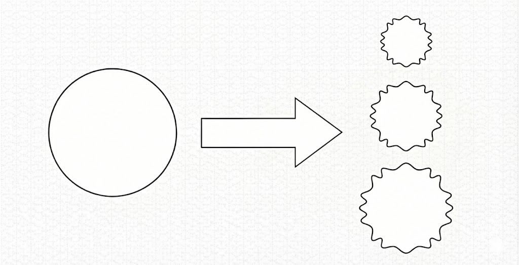
If your retrofit does not perform well (especially if you are already using self-distillation, plus maybe architecture-space graduality), a good question to ask is: how expressive is my changed architecture compared to the original architecture? This can help you understand how much you can expect the original model’s performance to be preserved, and what you could change to achieve higher performance.
I think of expressivity in very rough terms as ‘the class of functions that our model can represent’. For example, naively transferring a subword-level language model to the byte-level (by only changing the tokenizer) makes the embedding matrix much smaller, from on the order of 100k rows to 256 rows. In smallish models, the embedding matrix accounts for a substantial fraction of the total parameters so we might expect a naive byte-level transferred model to perform a lot worse in this case. Having fewer learnable parameters makes it less expressive. It is possible to devise a mechanism to retain the original embedding matrix to resolve this expressivity mismatch and improve performance.
Let’s take another example from retrofitting to the byte-level (completely coincidentally, this is where my own work is!). We can create a competitive byte-level retrofit by introducing a two-stage hierarchy with bytes as the first level and patches of one or more bytes as the second level as we did in Bolmo. How we group bytes into patches is quite important, and we saw that prior mechanisms to do so were less expressive than the subword tokenization mechanism used in the original model. Resolving this expressivity mismatch improved performance a lot.
There are also many examples outside of tokenization, for example from MOHAWK, which replaces Attention layers with SSMs to speed up the model, keeping Attention in a couple of layers to retain sufficient expressivity and (again) quantization, which vastly reduces the theoretical expressivity but empirically can be designed to mostly preserve the expressivity of the space LLM computations are in.
All in all, mismatches in the expressivity of the original and the retrofitted model can often explain performance differences. Sometimes, expressivity mismatches are desired, such as when creating a retrofit which should be faster than the original model by being less expressive. In other cases, they are bugs which we can fix to improve retrofitting performance.
Data Coverage
Dread it. Run from it. In the end you can’t escape making data choices. This is also true for retrofitting. What makes data tricky in the case of retrofitting is that we typically have a training budget which is orders of magnitude smaller than if we were to train from scratch. So we can only put so much data through the model. This can lead to worse behaviour on the tail ends of the distribution, even if we do a good job at preserving or improving performance on the bulk of the distribution’s mass.
I believe self-distillation helps here by making training somewhat less liable to overfit to the small extra portion of data that the model sees during the retrofitting phase, and by implicitly transferring some amount of tail-end knowledge through the distillation objective. That said, data is still extremely important, and there seems to be a disproportionally low amount of research done on data for retrofitting. I would love to see more work on it.
The best you can currently do, in my experience, is to choose a data mix which is close to the data the model is pretrained on, but potentially a higher-quality subset. For example, mid-training datasets like Dolmino are likely to be a good fit. The reason to choose a higher-quality subset is that we don’t need nearly the same volume of data as when we pre-train. However, this decision might also negatively impact tail-end performance due to less data diversity, so there is (again) no free lunch.
A data anecdote from Bolmo might help illustrate some of the interesting directions data research could take: we didn’t explicitly prioritise maths performance, so the fraction of maths data in our mix was relatively small (but nonzero). In hindsight, unsurprisingly, maths is the one area where in our benchmarks Bolmo is substantially behind the original model. This is still a good outcome. We have a benchmark for maths and we know that maths performance is worse. But there could be other areas where some aspect of the architecture change caused a performance degradation which we are not aware of. I would be very curious if there are effective ways to automatically identify these kinds of problem areas during training without explicit benchmarks to track them. But for now, the best we can do is to carefully design our data mix.
Conclusion
To summarise: if you’re retrofitting a model, start with self-distillation. This is the single most impactful ingredient. Then consider whether your architecture change is drastic enough to warrant graduality, check for expressivity mismatches that might limit your ceiling, and think carefully about data coverage.
I’m excited to see more work on retrofitting! It can be a powerful tool complementary to training from scratch, without being nearly as expensive. If you try these ingredients on your own project, I’d love to hear how it goes.
Acknowledgments
Thanks to Hannah Sterz and Auss Abbood for feedback on a draft of this post.